


 Equity management

 Equity management
- Fund management

 Fund management
 - Fund managementFund management
- Fund managementFund management




As a startup founder, you are likely to consider using stock options, whether it be European options or American options, when structuring employee incentives or raising funds. Valuing these options accurately is essential, and that is where the Black-Scholes Model becomes invaluable.
This mathematical finance tool calculates the theoretical price of a call option as well as the price of a put option. It was created by economists Fischer Black and Myron Scholes in the early 1970s. The model's influence was so profound that Myron Scholes and Robert Merton, who later refined it, received the 1997 Nobel Prize in Economics. Fischer Black's work was honored after his passing.
It is considered a benchmark in quantitative finance and remains essential for anyone working with equity-based compensation. For you, the Black-Scholes Model matters because it helps estimate the fair value of stock options based on measurable variables like the price of the underlying asset. This blog will guide you through its core principles, reveal the assumptions it relies on, and weigh its real-world uses against its limits.
To truly appreciate the significance of the Black-Scholes Model, you need to understand the financial landscape that gave birth to it. In the late 1960s and early 1970s, option markets were undergoing significant changes. Options trading was gaining popularity, but no one had a reliable method to determine the pricing of options accurately. Traders depended on intuition or basic approximations, which often led to inconsistent and risky decisions.
Fischer Black and Myron Scholes developed the model in 1973, addressing this gap with their groundbreaking work published in the Journal of Political Economy. Black, with his background in mathematical finance, collaborated with Scholes, an economist skilled in market dynamics, to create a formula rooted in the theory of options pricing. Their work built on the theory of rational option pricing. Robert Merton independently enhanced the model with insights published in the Bell Journal of Economics and Management Science in 1973. His contributions were so crucial that the model is often called the Black-Scholes-Merton Model.
After Black and Scholes published their findings, the industry adopted their method quickly, boosting the development of modern options exchanges like the Chicago Board Options Exchange, which opened in 1973. Their work earned Scholes and Merton the 1997 Nobel Prize in Economics, though Fischer Black had passed away in 1995. His contributions, however, remain integral to the model's enduring value.
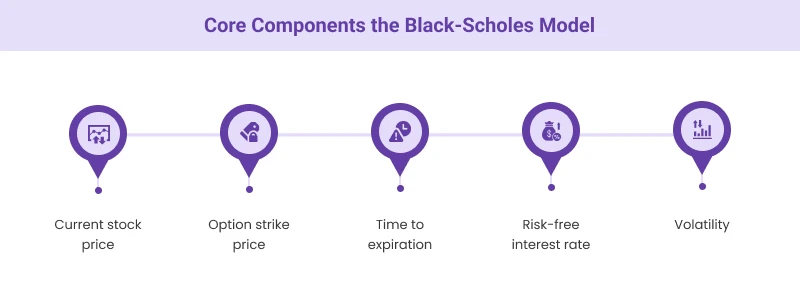
Here are the five core components the Black-Scholes Model uses to determine the fair price of an option:
1. Current stock price: This is the market price of the stock today. The Black-Scholes Model starts here because it reflects the real-time value an option is tied to. A higher current price typically increases the option's value.
2. Option strike price: This is the fixed price at which the option holder can buy or sell your stock. The model compares this to the current stock price to assess whether the option is profitable.
3. Time to expiration: Options have a deadline, usually measured in trading days. The longer the time period until expiration, the more opportunity there is for your stock price to move, which the Black-Scholes Model factors into its pricing.
4. Risk-free interest rate: This reflects the rate of return on a safe investment, like a U.S. Treasury bill. The model uses it as a discount factor to account for the time value of money, impacting how your option's price evolves.
5. Volatility: This measures how much your stock price fluctuates, often expressed as the standard deviation. Higher volatility of the underlying asset means greater uncertainty, increasing an option's potential value.
The Black-Scholes Model relies on specific assumptions to work effectively, and you need to understand them to use it wisely.
1. Efficient markets: The model assumes that markets are efficient and that asset prices follow a geometric Brownian motion, a random pattern driven by a differential equation. This means past price changes can't predict the direction of the market.
2. Constant volatility: The model assumes that the volatility of the underlying stock remains constant over the option's life. However, this might not be realistic for a rapidly growing or changing startup.
3. No transaction costs or taxes: The model assumes that there are no transaction costs or taxes involved in buying or selling the option or the underlying asset.
4. Log-normal distribution of stock prices: The model assumes that asset prices follow a lognormal distribution, reflecting positive price movements over time.
5. No-arbitrage conditions: The model assumes there are no risk-free arbitrage opportunities. This means that you can't make a guaranteed profit by simultaneously buying and selling related securities.
6. Risk-free interest rate: The model assumes that the risk-free interest rate is known and constant over the life of the option.
The formula calculates the current value of an option by combining probabilities with present value calculations. It uses inputs such as stock price, strike price, time to expiry, volatility, and interest rate. These elements work together to produce a result that reflects the likely value of the option at expiry.
The Black-Scholes formula for a call option is:
C = S * N(d1) - K * e^(-rt) * N(d2)
Here:
C = Call option price
S = Current stock price
K = Strike price of the option
r = Risk-free interest rate
t = Time to option expiration
N = Cumulative distribution function of the standard normal distribution
e = Exponential term (2.71828)
And d1 and d2 are calculated as:
d1 = [ln(S/K) + (r + σ^2/2)t] / (σ√t)
d2 = d1 - σ√t
Where:
σ (sigma) = Volatility of the underlying stock
Let’s examine each component:
Once you have input all the variables and run the Black-Scholes model, you will get a theoretical price for the option. Here is all about what this number actually means for your company:
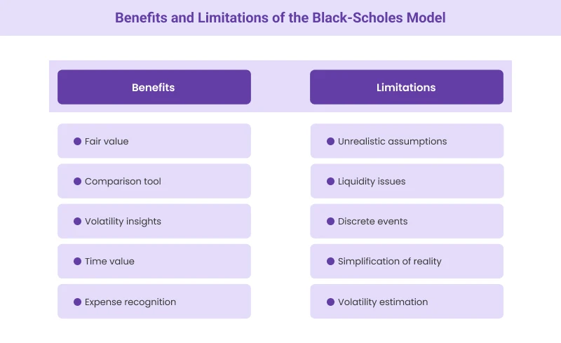
1. Fair value: The output of the Black-Scholes model represents the theoretical fair value of the option. If you are granting stock options to employees, this value can help understand the potential cost to your company.
2. Comparison tool: You can use this value to compare different option structures. For example, you might consider how changing the expiration date or strike price affects the option's value.
3. Volatility insights: If the market price of similar options differs significantly from your calculated price, it might indicate that the market's expectation of your company's volatility is different from your assumption.
4. Time value: The difference between the option's price and its intrinsic value (the amount by which it's in-the-money) represents its time value. This can help you understand how much of the option's value comes from the potential for future price movements.
5. Expense recognition: For accounting purposes, the fair value calculated by the Black-Scholes model is often used to determine the expense that needs to be recognized when granting stock options.
Here are some key benefits of using the Black-Scholes Model:
1. Standardization: The Black-Scholes model provides a standardized approach to option pricing. This means you can easily compare different option structures and communicate their value to investors, employees, and other stakeholders.
2. Efficiency: Once you understand the inputs, you can quickly calculate option values using readily available software or online calculators. This efficiency is crucial for making rapid decisions about equity compensation.
3. Risk management: The model helps you quantify the potential cost of offering stock options, allowing for better financial planning and risk management.
4. Theoretical foundation: The Black-Scholes model is built on solid financial theory. This gives you a strong basis for defending your valuation decisions if questioned by investors or auditors.
5. Versatility: While originally developed for financial options, the model can be adapted to value real options in business strategy, helping you assess the value of future opportunities for your startup beyond the stock market.
While the Black-Scholes model is powerful, it's not without its limitations:
1. Unrealistic assumptions: The model assumes constant volatility and a normal distribution of returns. This often does not hold true in real markets, especially for startups with potentially volatile growth.
2. Liquidity issues: The model assumes perfect liquidity, which may not apply to your startup's stock, especially in the early stages.
3. Discrete events: The model does not account for sudden and large price movements that can occur due to major company announcements.
4. Simplification of reality: It does not consider factors like taxes, transaction costs, or changing interest rates, which can affect option values.
5. Volatility estimation: For startups, estimating future volatility can be challenging, potentially leading to inaccurate valuations.
To address these gaps, newer models have been introduced. Alternatives like the Binomial Option Pricing Model or Monte Carlo simulations offer more flexibility by considering changing market conditions or non-linear behavior. Knowing these alternatives helps you apply more accurate pricing frameworks, especially when your startup's financial landscape doesn't match standard assumptions.
Over the years, the financial industry has made several modifications to improve the accuracy of the Black Scholes model:
1. Implied volatility: Instead of using historical volatility, many traders now use implied volatility derived from market prices to account for future expectations.
2. Stochastic volatility models: These allow for changing volatility over time, providing a more realistic representation of market conditions.
3. Jump-diffusion models: These account for sudden price movements that the original model does not consider.
4. Fractional Brownian motion: This adaptation allows for long-term dependencies in price movements, addressing the limitation of the random walk assumption.
The Black-Scholes Model has found widespread application in various areas of finance. Here is how it's used in real-world scenarios:
1. Options trading: Traders use the model to price options and develop trading strategies. It helps them identify potentially overvalued or undervalued options in the market.
2. Risk management: Financial institutions use the model to assess and hedge their risk exposure to various financial instruments.
3. Corporate finance: Companies use it to value warrants, convertible securities, and employee stock options. It is a crucial tool in designing executive compensation packages.
4. Mergers and acquisitions: The model helps in valuing complex financial structures often involved in M&A deals.
5. Real options analysis: Some companies adapt the model to value real business opportunities, like the option to expand into a new market or develop a new product.
For startup founders like you, one of the most relevant applications of the Black-Scholes Model is in valuing Employee Stock Options (ESOs). The experts at Qapita use this model as part of our equity management solutions to help startups navigate the complex calculations related to stock options.
Here is why the Black-Scholes Model is crucial for ESO valuation:
1. Accounting standards: Financial reporting standards (like ASC 718 in the US) require companies to expense the fair value of stock options. The Black-Scholes Model is widely accepted for calculating this fair value.
2. Transparency: A standardized model like Black-Scholes provides employees with transparency about the potential value of their options. This can be a powerful tool for attracting and retaining talent.
3. Investor communications: When raising funds, investors will want to understand your company's equity structure. A Black-Scholes valuation of your outstanding options can provide clarity and credibility.
4. Tax implications: In some jurisdictions, the fair value of options at grant can have tax implications. An accurate valuation is crucial for both the company and the employees.
5. Scenario planning: The model allows you to run different scenarios (e.g., different vesting schedules or strike prices) to optimize your equity compensation strategy.
However, applying the Black-Scholes Model to ESOs is not straightforward. Here are some challenges you might face:
1. Volatility estimation: As a private company, you don't have historical stock price data to estimate volatility. You might need to use data from comparable public companies or make educated guesses.
2. Expected term: ESOs often have complex vesting schedules and exercise behavior that differs from standard options. You might need to adjust the ‘time to expiration' input.
3. Dividends: While many startups don't pay dividends, if you plan to in the future, this needs to be factored into the model.
4. Illiquidity: Unlike publicly traded options, ESOs can't be easily sold or transferred. Some companies apply a discount to the Black-Scholes value to account for this.
At Qapita, we have developed advanced platforms that perform these calculations and help manage the entire lifecycle of your company's equity. Our equity management platform can help you:
The Black Scholes model has shaped the way global financial markets operate. Its introduction brought a more structured approach to pricing options, making it easier for institutions and investors to manage complex derivatives. As a founder, you may not be involved in daily trading, but the model's influence is visible across financial tools that affect your business indirectly.
It helped establish risk management practices that continue to guide portfolio strategies today. Banks, hedge funds, and institutional investors rely on it to forecast outcomes and manage exposure to market volatility. It also played a key role in the growth of the derivatives market by making these instruments more accessible and standardized.
Beyond trading desks, the model has influenced financial regulation by setting benchmarks for transparency in option pricing. Its structured framework helped shape valuation norms that are now commonly followed in corporate finance, especially when companies issue stock-based compensation or design capital allocation strategies.
The digital revolution has significantly enhanced the application and accessibility of the Black-Scholes Model. Here is how technology is shaping its use:
1. High-frequency trading: Algorithms based on the Black-Scholes Model now execute trades in milliseconds, increasing market efficiency. This rapid price discovery can affect how quickly information about your startup is reflected in related financial instruments.
2. Cloud computing: Cloud-based platforms now offer Black-Scholes calculations as a service, making sophisticated option pricing accessible to startups without significant IT investment.
3. Big data analytics: Advanced data analysis techniques are improving volatility predictions, a key input for the Black-Scholes Model. This could lead to more accurate valuations of your startup's options.
4. Machine learning: AI algorithms are being used to enhance the Black-Scholes Model, potentially addressing some of its limitations. This could help ensure accurate pricing of complex options structures in the future.
The Black Scholes model continues to play a vital role in financial decision-making, especially when it comes to option pricing and equity valuation. As a founder, understanding how this model supports transparency and consistency in valuing employee stock options can help you build a more structured equity strategy.
At Qapita, we help you manage this complexity with ease. Our platform, rated as #1 by G2, simplifies equity management by offering advanced valuation tools that incorporate models like Black-Scholes to deliver accurate and audit-ready outcomes. Whether you are issuing new grants, planning ESOP allocations, or preparing for a funding round, we ensure your valuations are defensible and aligned with market standards.
We also offer liquidity solutions through our Marketplace, ensuring your team benefits from their ownership. Book a 1:1 demo with our experts today to learn more about our solutions.